ChipSeq analysis
Required modules (NYUAD-Dalma)
The software modules at NYUAD's HPC (Dalma) have been grouped according to analysis disciplines. For this tutorial, you will need the following modules.
module load gencore/1
module load gencore_qc/1.0
module load gencore_epigenetics/1.0
Required software
Once the modules are loaded, all the required software will be available for you. Below is a specific list of the software that we will be using for this tutorial and the links to the software pages.
Macs2 - https://github.com/taoliu/MACS
Introduction
ChiP-seq combines chromatin immunoprecipitation with high throughput sequencing and is used to analyze protein interaction with DNA and identify their binding sites. Understanding how proteins bind (e.g. looking at transcription factor binding and histone modifications) helps in understanding how genes (and ultimately phenotypes) are regulated and affected. ChipSeq falls under the epigenetic analysis category, and similar to other analysis categories, they involve a range of applications, tools and methods, which are all available to NYUAD HPC users by loading the gencore_epigenetics/1.0 module.
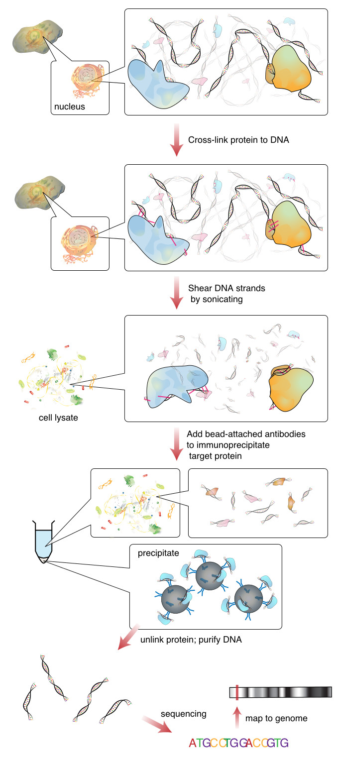
The image below outlines a typical ChipSeq preparation workflow,
In this tutorial, we will analyze data produced from a histone modification Chip-seq experiment, focusing on KO and WT conditions. We will specifically look for enrichment peaks through a process called "Peak calling", using a popular tools called MACS2.
Before we get started, you will find below some guidelines/considerations that relate to ChiP-seq analysis QC and data generation (sequencing).
ChiP-seq considerations
Sequencing approach & QC
Effective analysis of ChIP-seq data requires sufficient coverage by sequence reads (sequencing depth). It mainly depends on the size of the genome, and the number and size of the binding sites of the protein.
- For mammalian transcription factors (TFs) and chromatin modifications such as enhancer-associated histone marks, 20 million reads are adequate (4 million reads for worm and fly TFs).
- Proteins with more binding sites (e.g., RNA Pol II) or broader factors: need more reads, up to 60 million for mammalian ChIPseq.
- Sequencing depth rules of thumb:
- >10M reads for narrow peaks
- >20M reads for broad peaks
- Long & paired-end reads useful but not essential
- Replicates are a good idea, but unlike RNA-Seq, more than 2 replicates does not significantly increase the number of targets.
- Control samples should be sequenced significantly deeper than the ChIP ones in a TF experiment and in experiments involving diffused broad-domain chromatin data.
- This ensures sufficient coverage of a substantial portion of the genome and non-repetitive autosomal DNA regions.
- Always check the quality of raw sequenced reads to determine the appropriate QC/QT steps. For example, marking duplicates rather than filtering them out is a better approach in ChiPseq experiments. However, if a substantial amount of raw reads PCR duplicates were flagged (by examining the FastQC report duplication levels), then it probably is a good idea to filter these out (Hint: PICARD tools MarkDuplicates can achieve this).
Read alignment
- When aligning to a reference genome, we are interested in the uniquely mapped reads. Again, a good measure of uniquely mapped reads is ~70% (of quality trimmed reads not raw reads) for mammalian genomes (human, mouse), however, this varies between genomes. Less than 50% might be a cause for concern.
- A low percentage of uniquely mapped reads might point towards high amplification (PCR) and/or sequencing bias (optical duplicates). In this case, revisit the QC reports.
- Peak callers tend to ignore multi-mapping reads during the peak calling algorithm stage.
Workflow walkthrough
For this exercise, we will be using Histone Chipseq data from the ENCODE project. The dataset is in the form of QC'ed and filtered BAM alignment files, and includes 2 replicates and 1 control. The data has been aligned to the mouse (mm10 genome release) genome reference, and is derived from H3K9me3 ChIP-seq on embryonic 10.5 day mouse heart samples. The ENCODE experiment identifier for the replicates is ENCSR455REA, and ENCSR681NQF for the control sample.
So, we have a total of 3 BAM files, and they are all named according to their ENCODE identifiers. Below, is a description of the files,
ENCFF128QRQ.bam ---- Control
ENCFF543QFQ.bam ---- Replicate 1
ENCFF596FFU.bam ---- Replicate 2
Peak calling (MACS2)
MACS2 (https://github.com/taoliu/MACS), is a popular tool when analyzing ChiPseq data. Below is a usage example for histone modification aligned datasets, given 1 replicate and 1 control (assuming the BAM alignments originate from the alignment of paired end sequenced data).
macs2 callpeak -t histoneChipseq-processed.bam -c input-processed.bam \
-n histone --outdir macs2/histone_peaks -f BAMPE -g 1.87e9 \
--fix-bimodal --broad --bdg
You should also see a file with a .r extension. This is an executable R script that you can use to plot "The peak model" and "Cross correlation" in pdf output,
cd /scratch/$USER/chipseq/macs2_callpeaks
Rscript histone_model.r
Next, we will examine the macs2 output, mainly the xls file and the Peaks files.
You can use FileZilla to copy the required files to your local machine.
Parameter summary
-t treatment filename.
-c control filename (Input in this case).
-n the prefix for output filenames.
--outdir path to output directory.
-f Input file format (BAMPE in this case because we have a BAM alignment file generated from paired end sequencing).
-g Effective genome size.
--fix-model Enable auto paired-peak processing.
--broad Call broad peaks (makes sense for histone modification data).
--bdg Store BegGraph output files.
--call-summits reanalyze the shape of signal profile (p or q-score depending on cutoff setting) to deconvolve subpeaks within each peak called from general procedure.
Exercise: Calling peaks from BAM alignment files
Retrieving the data and preparing your environment
Open a terminal window and log in to Dalma
ssh $USER@dalma.abudhabi.nyu.edu
Start an interactive session
srun --mem 20GB --time 04:00:00 --pty /bin/bash

cd /scratch/$USER
Checking the size of the dataset directory
du -sh /scratch/gencore/January_workshop/chipseq/
As you can see, the folder size is large, so instead of copying the data, we will create a symbolic link (or a pointer) to the data.
First, create a chipseq folder in your scratch directory,
mkdir /scratch/$USER/chipseq
cd /scratch/$USER/chipseq
mkdir data
Now link the data directory,
ln -s /scratch/gencore/January_workshop/chipseq/data/ENCFF128QRQ.bam data/
ln -s /scratch/gencore/January_workshop/chipseq/data/ENCFF543QFQ.bam data/
ln -s /scratch/gencore/January_workshop/chipseq/data/ENCFF596FFU.bam data/
Next, load the appropriate modules,
module load gencore
module load gencore_epigenetics
module load gencore_variant_detection
Retrieving basic alignment statistics with bamtools
In this section, we will use bamtools to index our alignment files and report some basic stats. Please refer to the software page for more details https://github.com/pezmaster31/bamtools/wiki
bamtools index -in data/ENCFF128QRQ.bam
bamtools index -in data/ENCFF543QFQ.bam
bamtools index -in data/ENCFF596FFU.bam
Get some basic alignment stats,
bamtools stats -in data/ENCFF128QRQ.bam
bamtools stats -in data/ENCFF543QFQ.bam
bamtools stats -in data/ENCFF596FFU.bam
Macs2
Invoke the macs2 help screen and look at the tools bundled with the software, and usage.
macs2 -h
Now look at the callpeak program of macs2 and its usage,
macs2 callpeak -h
Now it is time to call peaks (this can take 30 mins),
macs2 callpeak -t data/ENCFF543QFQ.bam data/ENCFF596FFU.bam \
-c data/ENCFF128QRQ.bam -n histone --outdir macs2_callpeaks/ \
-g 1.87e9 --fix-bimodal --broad --tempdir /scratch/$USER/tmp/ --bdg
Or
macs2 callpeak -t data/ENCFF543QFQ.bam data/ENCFF596FFU.bam \
-c data/ENCFF128QRQ.bam  -B --nomodel --extsize 147 --SPMR \
-g mm -n histone_mod --outdir macs2_callpeaks_no_broad --tempdir /scratch/$USER/tmp/ --bdg
Question: What do the different parameters do is each example? (Hint: Use the help menu "macs2 callpeak -h").
Question: Given what you know about the dataset you are analyzing, which execution of callpeak makes more sense?
Visualizing the output from both commands can help further determine the effects of parameter choice.
Generate fold-enrichment using bdgcmp,
cd macs2_callpeaks/
macs2 bdgcmp -t histone_treat_pileup.bdg -c histone_control_lambda.bdg -o histone_FE_bdgcmp.bdg -m FE
Summary of output files
We will now examine the output files from the peak calling exercise. For your reference, below is a summary (from the Macs2 website) regarding the output files that are produced from Macs2 callpeak.
NAME_peaks.xls is a tabular file which contains information about called peaks. You can open it in excel and sort/filter using excel functions. Information include:
- chromosome name
- start position of peak
- end position of peak
- length of peak region
- absolute peak summit position
- pileup height at peak summit, -log10(pvalue) for the peak summit (e.g. pvalue =1e-10, then this value should be 10)
- fold enrichment for this peak summit against random Poisson distribution with local lambda, -log10(qvalue) at peak summit
Coordinates in XLS is 1-based which is different with BED format.
NAME_peaks.narrowPeak is BED6+4 format file which contains the peak locations together with peak summit, pvalue and qvalue. You can load it to UCSC genome browser. Definition of some specific columns are:
- 5th: integer score for display
- 7th: fold-change
- 8th: -log10pvalue
- 9th: -log10qvalue
- 10th: relative summit position to peak start
The file can be loaded directly to UCSC genome browser. Remove the beginning track line if you want to analyze it by other tools.
NAME_summits.bed is in BED format, which contains the peak summits locations for every peaks. The 5th column in this file is -log10pvalue the same as NAME_peaks.bed. If you want to find the motifs at the binding sites, this file is recommended. The file can be loaded directly to UCSC genome browser. Remove the beginning track line if you want to analyze it by other tools.
NAME_peaks.broadPeak is in BED6+3 format which is similar to narrowPeak file, except for missing the 10th column for annotating peak summits.
NAME_peaks.gappedPeak is in BED12+3 format which contains both the broad region and narrow peaks. The 5th column is 10*-log10qvalue, to be more compatible to show grey levels on UCSC browser. Tht 7th is the start of the first narrow peak in the region, and the 8th column is the end. The 9th column should be RGB color key, however, we keep 0 here to use the default color, so change it if you want. The 10th column tells how many blocks including the starting 1bp and ending 1bp of broad regions. The 11th column shows the length of each blocks, and 12th for the starts of each blocks. 13th: fold-change, 14th: -log10pvalue, 15th: -log10qvalue. The file can be loaded directly to UCSC genome browser.
NAME_model.r is an R script which you can use to produce a PDF image about the model based on your data. Load it to R by:
``Rscript NAME_model.r```
Then a pdf file NAME_model.pdf will be generated in your current directory. Note, R is required to draw this figure.
The .bdg files are in bedGraph format which can be imported to UCSC genome browser or be converted into even smaller bigWig files. There are two kinds of bdg files: treat_pileup, and control_lambda.
Visualizing the data with IGV
Finally, let's see what our ChiP experiment looks like! Here we will use IGV to visualize the peaks between the two conditions. Another common approach is to use the UCSC genome browser, a good tutorial on this can be found on https://genome.ucsc.edu/goldenPath/help/customTrack.html